Build nanoGPT

[Code] of the project

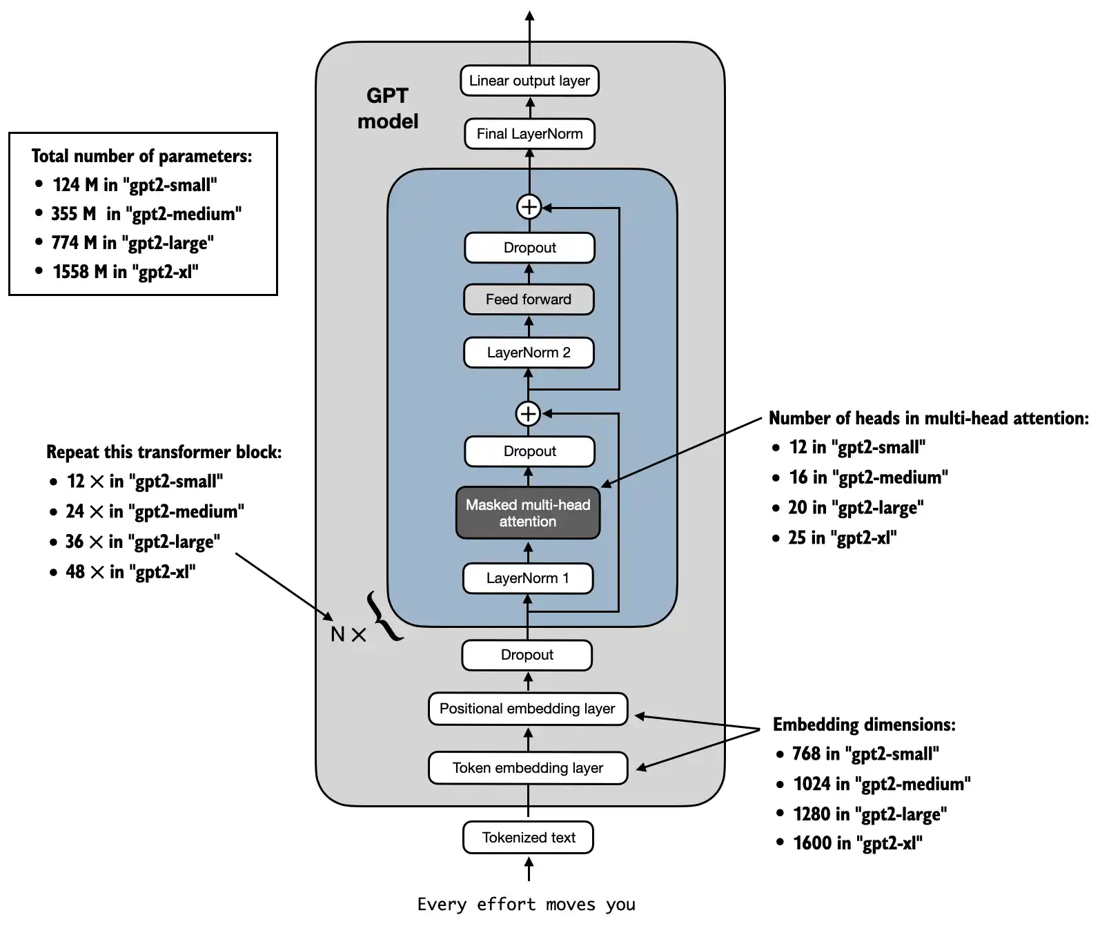
GPT-2架构

本次我们复现的是其124M结构模型^[1][3] (openai 采用out_head和token_emb层共享参数)

GPT_CONFIG_124M = {
           "vocab_size": 50257,     # Vocabulary size
           "context_length": 1024,  # Context length
           "emb_dim": 768,          # Embedding dimension
           "n_heads": 12,           # Number of attention heads
           "n_layers": 12,          # Number of layers
           "drop_rate": 0.1,        # Dropout rate
           "qkv_bias": False        # Query-key-value bias
       }

GPTModel

• tokenizer
• transformer block * n
• out_head

class GPTModel(nn.Module):
    def __init__(self, cfg):
        super().__init__()
        self.tok_emb = nn.Embedding(cfg["vocab_size"], cfg["emb_dim"])
        self.pos_emb = nn.Embedding(cfg["context_length"], cfg["emb_dim"])
        self.drop_emb = nn.Dropout(cfg["drop_rate"])
        self.cfg = cfg

        self.trf_blocks = nn.Sequential(
            *[TransformerBlock(cfg) for _ in range(cfg["n_layers"])])

        self.final_norm = LayerNorm(cfg["emb_dim"])
        self.out_head = nn.Linear(cfg["emb_dim"], cfg["vocab_size"], bias=False)
        self.tok_emb.weight = self.out_head.weight  # weight tying
        self.apply(self._init_weights) # Initialize weights


    def _init_weights(self, module):
        if isinstance(module, nn.Linear):
            std = 0.02
            if hasattr(module, 'NANOGPT_SCALE_INIT'):
                std *= (2 * self.cfg["n_layers"]) ** -0.5
            torch.nn.init.normal_(module.weight, mean=0.0, std=std)
            if module.bias is not None:
                torch.nn.init.zeros_(module.bias)
        elif isinstance(module, nn.Embedding):
            torch.nn.init.normal_(module.weight, mean=0.0, std=0.02)

    def forward(self, in_idx):
        batch_size, seq_len = in_idx.shape
        tok_embeds = self.tok_emb(in_idx)
        pos_embeds = self.pos_emb(torch.arange(seq_len, device=in_idx.device))
        x = tok_embeds + pos_embeds  # Shape [batch_size, num_tokens, emb_size]
        x = self.drop_emb(x)
        x = self.trf_blocks(x)
        x = self.final_norm(x)
        logits = self.out_head(x)
        return logits

Transformerblock

class TransformerBlock(nn.Module):
    def __init__(self, cfg):
        super().__init__()
        self.att = MultiHeadAttention(
            d_in=cfg["emb_dim"],
            d_out=cfg["emb_dim"],
            context_length=cfg["context_length"],
            num_heads=cfg["n_heads"],
            dropout=cfg["drop_rate"],
            qkv_bias=cfg["qkv_bias"])
        self.ff = FeedForward(cfg)
        self.norm1 = LayerNorm(cfg["emb_dim"])
        self.norm2 = LayerNorm(cfg["emb_dim"])
        self.drop_shortcut = nn.Dropout(cfg["drop_rate"])

    def forward(self, x):
        # Shortcut connection for attention block
        shortcut = x
        x = self.norm1(x)
        x = self.att(x)   # Shape [batch_size, num_tokens, emb_size]
        x = self.drop_shortcut(x)
        x = x + shortcut  # Add the original input back

        # Shortcut connection for feed-forward block
        shortcut = x
        x = self.norm2(x)
        x = self.ff(x)
        x = self.drop_shortcut(x)
        x = x + shortcut  # Add the original input back

        return x

Layernorm:

class LayerNorm(nn.Module):
    def __init__(self, emb_dim):
        super().__init__()
        self.eps = 1e-5
        self.scale = nn.Parameter(torch.ones(emb_dim))
        self.shift = nn.Parameter(torch.zeros(emb_dim))

    def forward(self, x):
        mean = x.mean(dim=-1, keepdim=True)
        var = x.var(dim=-1, keepdim=True, unbiased=False)
        norm_x = (x - mean) / torch.sqrt(var + self.eps)
        return self.scale * norm_x + self.shift

Gelu:

class GELU(nn.Module):
    def __init__(self):
        super().__init__()

    def forward(self, x):
        return 0.5 * x * (1 + torch.tanh(
            torch.sqrt(torch.tensor(2.0 / torch.pi)) *
            (x + 0.044715 * torch.pow(x, 3))
        ))

其中前向传播网络由三层组成：

class FeedForward(nn.Module):
    def __init__(self, cfg):
        super().__init__()
        self.layers = nn.Sequential(
            nn.Linear(cfg["emb_dim"], 4 * cfg["emb_dim"]),
            GELU(),
            nn.Linear(4 * cfg["emb_dim"], cfg["emb_dim"]),
        )
        self.layers[-1].NANOGPT_SCALE_INIT = True # Special flag for weight initialization

    def forward(self, x):
        return self.layers(x)

• 注意：NANOGPT_SCALE_INIT = True是为了与openai初始化权重时一致而添加的一个特殊标志位，下节会具体讲解

多头注意力：

class MultiHeadAttention(nn.Module):
    def __init__(self, d_in, d_out, context_length, dropout, num_heads, qkv_bias=False):
        super().__init__()
        assert d_out % num_heads == 0, "d_out must be divisible by n_heads"

        self.d_out = d_out
        self.num_heads = num_heads
        self.head_dim = d_out // num_heads  # Reduce the projection dim to match desired output dim

        self.W_query = nn.Linear(d_in, d_out, bias=qkv_bias)
        self.W_key = nn.Linear(d_in, d_out, bias=qkv_bias)
        self.W_value = nn.Linear(d_in, d_out, bias=qkv_bias)
        self.out_proj = nn.Linear(d_out, d_out)  # Linear layer to combine head outputs
        
        self.out_proj.NANOGPT_SCALE_INIT = True  # Special flag for weight initialization

        self.dropout = nn.Dropout(dropout)
        self.register_buffer('mask', torch.triu(torch.ones(context_length, context_length), diagonal=1))

    def forward(self, x):
        b, num_tokens, d_in = x.shape

        keys = self.W_key(x)  # Shape: (b, num_tokens, d_out)
        queries = self.W_query(x)
        values = self.W_value(x)

        # We implicitly split the matrix by adding a `num_heads` dimension
        # Unroll last dim: (b, num_tokens, d_out) -> (b, num_tokens, num_heads, head_dim)
        keys = keys.view(b, num_tokens, self.num_heads, self.head_dim)
        values = values.view(b, num_tokens, self.num_heads, self.head_dim)
        queries = queries.view(b, num_tokens, self.num_heads, self.head_dim)

        # Transpose: (b, num_tokens, num_heads, head_dim) -> (b, num_heads, num_tokens, head_dim)
        keys = keys.transpose(1, 2)
        queries = queries.transpose(1, 2)
        values = values.transpose(1, 2)

        # Compute scaled dot-product attention (aka self-attention) with a causal mask
        attn_scores = queries @ keys.transpose(2, 3)  # Dot product for each head

        # Original mask truncated to the number of tokens and converted to boolean
        mask_bool = self.mask.bool()[:num_tokens, :num_tokens]

        # Use the mask to fill attention scores
        attn_scores.masked_fill_(mask_bool, -torch.inf)

        attn_weights = torch.softmax(attn_scores / keys.shape[-1]**0.5, dim=-1)
        attn_weights = self.dropout(attn_weights)

        # Shape: (b, num_tokens, num_heads, head_dim)
        context_vec = (attn_weights @ values).transpose(1, 2)

        # Combine heads, where self.d_out = self.num_heads * self.head_dim
        context_vec = context_vec.reshape(b, num_tokens, self.d_out)
        context_vec = self.out_proj(context_vec)  # optional projection

        return context_vec

至此，GPT-2的整个架构已经实现完毕啦

Training Techs

掌握训练模型时的必备技巧不仅能大大提高训练速度，也能助于提升性能

权重初始化(_init_weights)

• 权重初始化一般符合正态分布，均值$u$为0，标准差$\sigma$为$\frac{1}{\sqrt{Dimension}}= \frac{1}{\sqrt{768}}=0.036$ (0.02是一个合理的值，因为我们这里复现的size是small)
• 对于有残差的网络模块，通常会额外增加一个乘积因子$\frac{1}{N}$来初始化权重为$\frac{1}{N*Dimension}$
  • 其中$N$是残差的次数

如下有个很好地解释

x = torch.zeros(768)
n = 100
for i in range(n):
	x += torch.randn(768) # 
print(x.std())

• 你会发现x从最初的0，增长到了$\sqrt{100}$左右，假设每个$\epsilon ∼N(0,1)$

• 根据方差的线性性质：

  $$\begin{align*} \text{Var}(x_i) &= \text{Var}\left(\sum_{j=1}^{n} z_{i,j}\right) \\ &= \sum_{j=1}^{n} \text{Var}(z_{i,j}) \\ &= n \end{align*}$$

  因此，x 的标准差为：

  $std(x)= \sqrt{n}$

• 故对于残差网络层（见上图TransfomerBlock架构，实际上就是多头注意力的最后一层和FFN的最后一层），我们需要额外设置因子来初始化权重。（2 * self.cfg["n_layers"]是因为一个transformerblock中有两个残差次数）

if hasattr(module, 'NANOGPT_SCALE_INIT'):
   std *= (2 * self.cfg["n_layers"]) ** -0.5

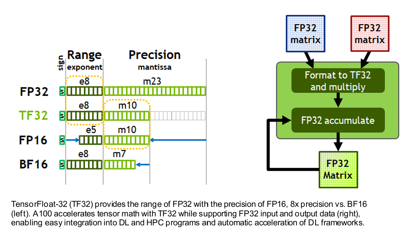
混合精度训练（Mixed Precision Training）

Nvidia官方详解：Nvidia-ampere-architecture-whitepaper

• TF32在内存中保持32位，计算时被裁剪精度降低
• BF16则在内存和计算中都使用16位

混合精度训练的核心思想是利用 低精度（如 bfloat16 或 float16）来加速计算，同时利用 高精度（如 float32）来存储权重，保持模型训练的稳定性。

默认地torch采用fp32精度, 虽然保持最高的精度，但导致训练速度很慢，且实际使用中没有必要使用fp32来训练。具体来讲，我们的输入，输出，权重都为fp32保持不变，但我们希望在训练时候的激活和权重尽量减小来提高训练速度。

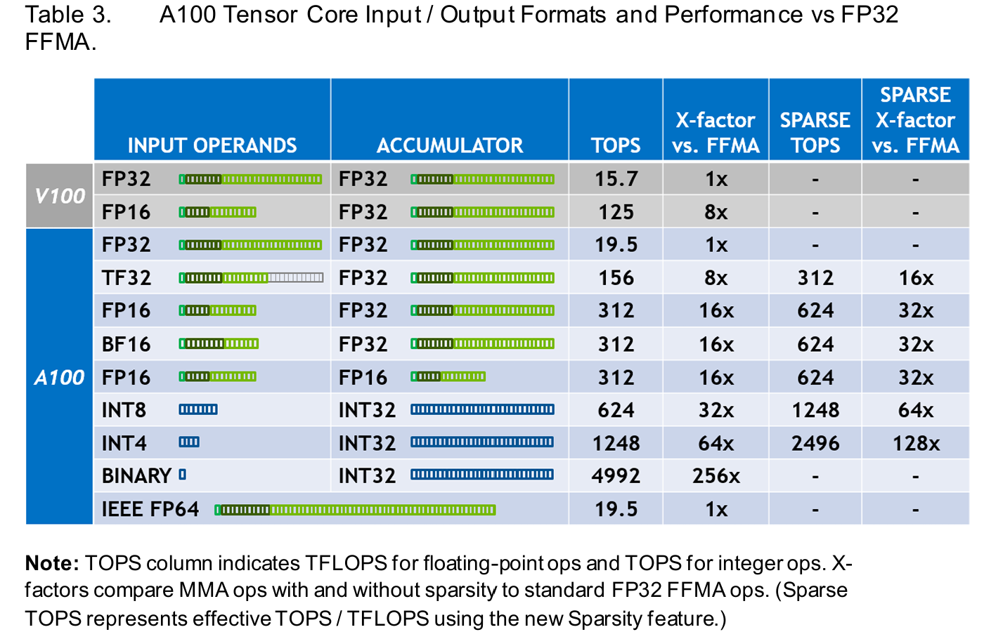
torch.set_float32_matmul_precision(precision)

• “highest”:
  • float32 数据类型进行矩阵乘法内部计算。
• “high”：
  • TensorFloat32 数据类型 (速度最大相比fp32可x8， 但实际碍于内存速率测试x3左右)
  • 或如果可用的快速矩阵乘法算法支持，可能会使用将 float32 视为两个 bfloat16 数字的和的策略
• “medium”：
  • bfloat16 数据类型进行矩阵乘法的内部计算（速度最大相比fp32可x16, 实际速度x3.5左右）

仅需额外增加一行代码，其他无需做任何修改。模型的权重都是fp32存储，不会改变，但计算矩阵乘积的时候却变为tf32，免费地大大提高训练速度！（该设置仅针对矩阵乘积有效）

代码示例：

torch.set_float32_matmul_precision("high")
for epoch in range(epochs):
    optimizer.zero_grad()  # Clear previous gradients
    logits = model(x)
    loss = F.cross_entropy(logits, y)
    loss.backward()
    optimizer.step()

autocasting

使用方式：将前向传播过程的计算logits和loss两个过程使用autocast包裹，backward使用默认精度反向传播

with torch.autocast(device_type=device_type, dtype=torch.bfloat16): # using bf16
    logits = model(input)
    loss = F.cross_entropy(logits.view(-1, logits.size(-1)),target.view(-1))
loss.backward()
optimizer.step()

• 实测比torch.set_float32_matmul_precision(precision)快一些

Torch.compile

默认情况下必须使用的技术

model = GPTModel(GPT_CONFIG_124M)
model.to(device)
model = torch.compile(model)

除非是debug，不然不用白不用，该项目中实测提升速度x3

Flashattention

默认情况下必须使用的技术，除非对于attention本身运算过程有所修改

torch.nn.Functional.scaled_dot_product_attention(queries, keys, values, is_causal=True, dropout_p=self.dropout_p)

class MultiHeadAttention(nn.Module):
    def __init__(self, d_in, d_out, context_length, dropout, num_heads, qkv_bias=False):
        super().__init__()
        assert d_out % num_heads == 0, "d_out must be divisible by n_heads"

        self.d_out = d_out
        self.num_heads = num_heads
        self.head_dim = d_out // num_heads  # Reduce the projection dim to match desired output dim

        self.W_query = nn.Linear(d_in, d_out, bias=qkv_bias)
        self.W_key = nn.Linear(d_in, d_out, bias=qkv_bias)
        self.W_value = nn.Linear(d_in, d_out, bias=qkv_bias)
        self.out_proj = nn.Linear(d_out, d_out)  # Linear layer to combine head outputs
        
        self.out_proj.NANOGPT_SCALE_INIT = True  # Special flag for weight initialization

        self.dropout = nn.Dropout(dropout)
        self.dropout_p = dropout
        self.register_buffer('mask', torch.triu(torch.ones(context_length, context_length), diagonal=1))

    def forward(self, x):
        b, num_tokens, d_in = x.shape

        keys = self.W_key(x)  # Shape: (b, num_tokens, d_out)
        queries = self.W_query(x)
        values = self.W_value(x)

        # We implicitly split the matrix by adding a `num_heads` dimension
        # Unroll last dim: (b, num_tokens, d_out) -> (b, num_tokens, num_heads, head_dim)
        keys = keys.view(b, num_tokens, self.num_heads, self.head_dim)
        values = values.view(b, num_tokens, self.num_heads, self.head_dim)
        queries = queries.view(b, num_tokens, self.num_heads, self.head_dim)

        # Transpose: (b, num_tokens, num_heads, head_dim) -> (b, num_heads, num_tokens, head_dim)
        keys = keys.transpose(1, 2)
        queries = queries.transpose(1, 2)
        values = values.transpose(1, 2)

        # # Compute scaled dot-product attention (aka self-attention) with a causal mask
        # attn_scores = queries @ keys.transpose(2, 3)  # Dot product for each head

        # # Original mask truncated to the number of tokens and converted to boolean
        # mask_bool = self.mask.bool()[:num_tokens, :num_tokens]

        # # Use the mask to fill attention scores
        # attn_scores.masked_fill_(mask_bool, -torch.inf)

        # attn_weights = torch.softmax(attn_scores / keys.shape[-1]**0.5, dim=-1)
        # attn_weights = self.dropout(attn_weights)

        # # Shape: (b, num_tokens, num_heads, head_dim)
        # context_vec = (attn_weights @ values)
        context_vec = F.scaled_dot_product_attention(queries, keys, values, is_causal=True, dropout_p=self.dropout_p)

        context_vec = context_vec.transpose(1, 2).contiguous().view(b, num_tokens, self.d_out)
        context_vec = self.out_proj(context_vec)  # optional projection

        return context_vec

• 速度x1.5，显存也有所减少

Lr scheduler

lr scheduler是调控学习率来提高模型的性能重要手段

warm up

• warm up的step一般为total_step的0.1%到20%

if it < configs.warmup_steps:
    return configs.max_lr * (it+1) / configs.warmup_steps

cosine decay

$$coeff=0.5×(1.0+cos(π×decay_{ratio}))$$

• 这个函数确保 coeff 从 1 开始，到训练结束时降到 0。

$$lr=minlr+coeff×(maxlr−minlr)$$

    # 3) in between, use cosine decay down to min learning rate
decay_ratio = (it - configs.warmup_steps) / (configs.max_steps - configs.warmup_steps)
assert 0 <= decay_ratio <= 1
coeff = 0.5 * (1.0 + math.cos(math.pi * decay_ratio)) # coeff starts at 1 and goes to 0
return configs.min_lr + coeff * (configs.max_lr - configs.min_lr)

最终：

def get_lr(it, configs):
    # 1) linear warmup for warmup_iters steps
    if it < configs.warmup_steps:
        return configs.max_lr * (it+1) / configs.warmup_steps
    # 2) if it > lr_decay_iters, return min learning rate
    if it > configs.max_steps:
        return configs.min_lr
    # 3) in between, use cosine decay down to min learning rate
    decay_ratio = (it - configs.warmup_steps) / (configs.max_steps - configs.warmup_steps)
    assert 0 <= decay_ratio <= 1
    coeff = 0.5 * (1.0 + math.cos(math.pi * decay_ratio)) # coeff starts at 1 and goes to 0
    return configs.min_lr + coeff * (configs.max_lr - configs.min_lr)

Distributed Data Parallel (DDP) for multiple GPUs training

torchrun 是 PyTorch 提供的一个命令行工具，用于启动和管理分布式训练

torchrun会自动初始化分布式环境，并为每个进程分配一个 rank 和 local_rank。除了rank不同，执行的代码完全一致。这些信息可以在代码中通过 os.environ['RANK'] 和 os.environ['LOCAL_RANK'] 获取。

• rank： 进程全局内独特的标号
  • gpu0: 0, gpu1: 1 .etc )
• local_rank： 进程在当前节点局部内的标号, 如果只有一个节点，那local_rank 和rank相等
• world_size：总进程数量

终端命令行

单节点运行^[2]：

torchrun
    --standalone
    --nnodes=1
    --nproc-per-node=$NUM_TRAINERS
    YOUR_TRAINING_SCRIPT.py (--arg1 ... train script args...)

• --standalone 使得分布式训练在单节点环境下运行，所有训练进程都在同一个节点上启动，而不需要通过多个节点进行通信。
• --nnodes=1 表示只有一个节点参与训练。
• --nproc-per-node 表示每个节点上启动的进程数。通常情况下，每个进程会绑定一个 GPU，所以 NUM_TRAINERS 通常等于要使用的 GPU 数量。

单节点多任务以及多节点运行查看torchrun官方文档

DDP代码过程

1. 初始化进程

• 在使用torchrun多GPU训练的代码中，第一步首先应该获取由torchrun传递的，当前进程的标识号rank，local_rank, 以及world_size。
• 保证cuda可用后，使用 init_process_group(backend="nccl", rank=rank, world_size=world_size)初始化分布式进程组
• 设置主进程以及当前进程的device

ddp_rank = int(os.environ.get('RANK', 0))
ddp_local_rank = int(os.environ['LOCAL_RANK'])
world_size = int(os.environ.get('WORLD_SIZE', 1))

assert torch.cuda.is_available(), "for now we need CUDA for DDP"


init_process_group(backend="nccl", rank=rank, world_size=world_size)

master_process = ddp_rank == 0 
device = f'cuda:{ddp_local_rank}'
device_type = "cuda" if device.startswith("cuda") else "cpu"
torch.cuda.set_device(device)

2. 将model使用DDP包裹, 同时保存原有的raw_model

from torch.nn.parallel import DistributedDataParallel as DDP
	model = DDP(model, device_ids=[ddp_local_rank])
    raw_model = model.moudle

• pytorch官方的文档对device_ids解释不清，但Andrej Karpathy^[1]很明确就是ddp_local_rank

• DDP的作用: 将每个节点每个step的loss.backward()反向传播同步，汇总求平均，每个节点保留平均梯度最后更新参数

• 但在本项目的实现中由于引进了grad_accum_steps, 希望loss累积不断addgrad_accum_steps后才进行梯度更新，因此需要额外利用require_backward_grad_sync控制DDP的梯度更新

• 对于原模型的保存，如果使用torch.compile，要在调用前就保存raw_model,否则参数名会带有前缀_orig_mod^[4]

for step in range(max_steps):
  for micro_step in range(grad_accum_steps):
      # only require sync on the last micro-step
      model.require_backward_grad_sync = (micro_step == grad_accum_steps - 1)

      input, target = train_loader.next_batch()
      input, target = input.to(device), target.to(device)
      logits = model(input)
      loss = F.cross_entropy(logits.view(-1, logits.size(-1)), target.view(-1))
      loss = loss / grad_accum_steps
      loss.backward() # 将loss反向传播累积，直到model.require_backward_grad_sync为True时，才进行梯度更新
   optimizer.step()
   lr_scheduler.step()

3. 分布式训练保存权重的方式^[5]

torch.save(raw_model.state_dict(), 'best_model.pth')

• 必须使用原模型保存权重，这样下次才能使用单卡GPU加载模型，而不是DDP多GPU加载

4. 训练结束释放分布式进程组

destroy_process_group()  # NEW: cleanly exit distributed mode

References

1. Andrejkarpathy, build-nanogpt: Video+code lecture on building nanoGPT from scratch https://github.com/karpathy/build-nanogpt ↩
2. torchrun (Elastic Launch) — PyTorch 2.6 documentation https://pytorch.org/docs/stable/elastic/run.html ↩
3. rasbt/LLMs-from-scratch: Implement a ChatGPT-like LLM in PyTorch from scratch, step by step https://github.com/rasbt/LLMs-from-scratch ↩
4. How to save/load a model with torch.compile - PyTorch Forums https://discuss.pytorch.org/t/how-to-save-load-a-model-with-torch-compile/179739 ↩
5. Hongyu Sun’s Blog: PyTorch save and load DDP model https://auniquesun.github.io/2022-04-13-pytorch-save-and-load-for-DDP-model/ ↩